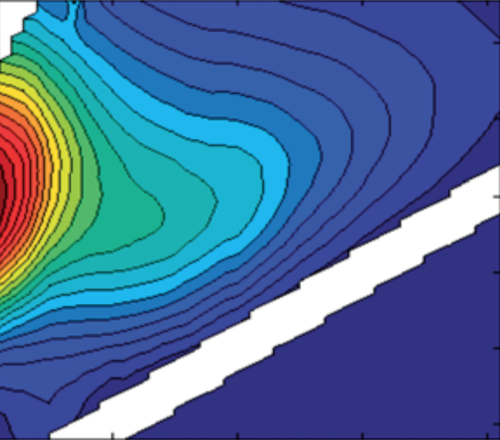
Plotting EEMs manually to get an overview
I had a request asking about some code that can plot EEMs manually to get an overview. Theoretically, eemview does this well, but can be quite complicated to use. This is in part due to the many customization requests/wishes by users making things complicated. So I thought I’d share a couple of lines of code with you that allow you to plot EEMs manually. The section of code below has some initial lines where options are defined. If you find yourself wanting more control, you can simply add a variable to control the behaviour of the loop below. Of course, this requires a bit more knowledge of Matlab than using eemview, but for those of you who have it, I’m sure this bit of code can be useful.
Note that I am not using subplot. Matlab has a new tilelayout function that can behave like subplot, but also offers much nicer automatic adaptation upon figure resizing if you set the tile layout with the flow option instead of specifying number of rows and columns.
The example below starts with two fully imported datasets that passed through checkdataset. My datasets always contain a cell array called filelist, so if you don’t have that, make sure to change the code below.
	eem=DS; % Change this. DS is the name of your dataset, eem is used to plot

	%% All the options here
	figureheight=20; % in centimeter
	figurewidth=30; % in centimeter
	n=1; % sample counter
	r=5; % number of rows (subplot)
	c=5; % number of columns (subplot)
	cnt=0; % figure counter.
	cntt=ceil(eem.nSample./(r*c)); % Total number of needed figures
	ncontours=10; % Number of contour lines
	ncolours=5; % Number of color contours
	xlimit=[min(eem.Ex) max(eem.Ex)]; % Change this if you want to
	ylimit=[min(eem.Em) max(eem.Em)]; % Change this if you want to
	clim=[0 max(eem.X(:),[],'omitnan')]; % Color limit. Change this how you like, e.g. nanmax(eem.X(:))
	manualcscale=false; % Do you want to use clim to scale the EEMs?
	saveeachfigure=false; % Do you want to save all the plots?

	%% Set the figure up
	fig=dreemfig; % Make a pretty figure with white background
	fig.Units="centimeters";
	Cpos=get(fig,'pos');
	set(fig,'pos', [Cpos(1) Cpos(2) figurewidth figureheight]);
	movegui(fig,'center');
	clearvars Cpos
	fig.Visible='off';drawnow

	%% Draw all the plots
	while n<eem.nSample
	    i=1;
	    t=tiledlayout(r,c,'TileSpacing','tight','Padding','loose');
	   while i<=r*c
	       if n>eem.nSample
	           break
	       end
	       nexttile(t)

	       contourf(eem.Ex,eem.Em,squeeze(eem.X(n,:,:)),ncolours,'LineStyle','none')
	       hold on
	       if manualcscale
	           contour(eem.Ex,eem.Em,squeeze(eem.X(n,:,:)),linspace(clim(1),clim(2),ncontours),'Color','k')
	       else
	           contour(eem.Ex,eem.Em,squeeze(eem.X(n,:,:)),ncontours,'Color','k')
	       end
	       if manualcscale
	          caxis(clim)
	       else
	           cb=colorbar;
	       end
	       xlim(xlimit)
	       ylim(ylimit)
	       title(eem.filelist{n})
	       i=i+1;
	       n=n+1;
	   end
	   if manualcscale
	       cb=colorbar;
	       cb.Layout.Tile = 'east';
	       ylabel(cb,'Fluorescence level')
	   end
	   drawnow
	   cnt=cnt+1;
	   ylabel(t,'Emission (nm)')
	   xlabel(t,'Exciatation (nm)')
	   title(t,['plot ',num2str(cnt),' of ',num2str(cntt)])
	   if saveeachfigure
		  exportgraphics(gcf,['eemoverview_',num2str(cnt),'.png'])
	   end
	   fig.Visible='on';
	   pause
	   fig.Visible='off';drawnow
	end
